Summary Book 1 - Chapter 6: Optimizing Parameters and Filtering Trading Signals

Quantitative trading strategies harnessing the power of quantitative techniques to create a winning trading program:


Optimization allows the trader to fine tune a strategy. however many believe fitting strategies to past data yields unrealistic expectations.

parameters are tweaked once a successful strategy is found. ex. Length of the moving average, the volatility multiplier.

to simplify the number of parameters we can use more than one unit per test. for example increment by five insread of one.

optimization is a technique to maximize the expected value of a trading strategy.

The first would use parameters for the current period that had performed best in the prior period. The idea behind this strategy is that strings of past performance are likely to continue, and that as traders we want to stay with parameter sets that are performing the best. The second test selected parameter sets for the current period that performed the worst in the prior period. The idea behind this strategy is that performance is likely to mean revert over time. Parameter sets that have been “cold” and performing poorly are likely to revert and perform well in the future.

avoid trend-following signals when futures are caught in trading ranges but to take trend-following signals when stocks are in trading ranges.

based on the ADX indicator we can select a specific strategy
ADX<15 RSI osscillator
ADX>25 Channel Breakout

Positive autocorrelation exists when greater than average values tend to lead to greater than average values in the next period, and vice versa. Negative autocorrelation exists when greater than average values lead to less than average values.

markets trend roughly 60 percent of the time. The fact that the average falls greater than 50 percent suggests that markets do in fact trend, and we can apply trend-following strategies to exploit this inefficiency.

Summary Book 1 - Chapter 3 Creating Trading Strategies

Quantitative trading strategies harnessing the power of quantitative techniques to create a winning trading program:

 3 building blocks for a trading system
1. Enteries - signals of buy and sell
2. Exits - indicate expected value of a trade has diminished to the point that the trade should be closed.
3. Filters - persuade the trader to only take entries with highest expected profits over the life of the system

Trend-following technique - buy signal while the market is in a period of strength.
sell signals are during period of weakness.

Moving average-the mean of a time series updated each trading day.
Most common moving averages are:Simple,Weighted, Exponential.

The simple moving average is an average of values recalculated every day.
Sum the previous days closing value and devide by the number of days.

Exponential moving average is calculated using todays price and yesterdays moving average value.alpha is the smoothing factor which is 2 devided by the number of days plus 1.

Sample Computation on EXCEL

A weighted moving average assigns higher weights to more recent data.

Trading signals are triggered when the price of a stock goes above the moving average, higher prices are likely and it signals that its time to buy.

When prices cross below the moving average, a declining market is expected and its time to sell.

a moving average of 20 to 100 days are commonly used to generate buy and sell signals. shorter moving averages will respond quicker to recent price movement.

longer moving averages produce trading signals infrequently.

when combining moving average methods such as exponential and simple, 10 and 40 days are used to generate signals.

if a market is prone to short and violent moves with many reversals along the way, moving average systems are likely to suffer. this drawback is called a whipsaw, asociated with choppy market action.

Channel breakout;
channels created when plotting a running tally of the highest highs and lowest lows over a fixed interval of days.

in a 40 day channel breakout: buy if market close was the highest of the past 40 days.
sell when the market close lower than any other close of the past 40 days.

A surge above the upper channel line shows extraordinary strength that can signal the start of an uptrend. Conversely, a plunge below the lower channel line shows serious weakness that can signal the start of a downtrend

Momentum-
take the difference between one value and another value at some point in time.
Momentum = Value Today - Value X days ago

Buy when todays close is greater than the close x days ago
Sell when todays close is less than the close x days ago

Volatility breakouts-
large short-term price jumps tend to be precursors of further movement in the same direction.
it is comprised of 3 pieces:
1. reference value - measurement price of the move from the start
2. volatility measure - computes the typical valatility of the market to separate significant movement from random price changes
3. volatility multiplier - determines the sensitivity of price movement required to trigger entry signals.

buy when prices close above the upper trigger.
sell when prices close below the lower trigger.

the most logical valatility measure is to calculate a standard deviation of price returns.

another volatility measure is to calculate the average true range.
1. the largest value of todays high minus todays low
2. largest value of todays high minus yesterdays close
3. largest value of yesterdays close minus todays low

 Excel Sheet showing how to calculate the 14 day Average True Range


average the true range over a set number of days to calculate ATR (average true range)

another volatility measure is the standard deviation of market prices.
this method does not allow strict interpretation using the normal distribution.

Volatility breakout entry points are derived by multiplying the volatility multiplier
by the volatility measure and adding that value to the reference value.

Volatility Breakout Rules
-Upper trigger = Reference Value (yesterday’s close, today’s open, short-term moving average) plus the Volatility Multiplier times Volatility Measure (standard deviation of price returns, average true range, standard deviation of
price). Buy when today’s close is greater than the upper trigger.
-Lower trigger = Reference Value (yesterday’s close, today’s open, short-term moving average) plus the Volatility Multiplier times Volatility Measure (standard deviation of price returns, average true range, standard deviation of
price). Sell when today’s close is less than the lower trigger

When a trend has become overextended or exhausted we define the technique as an Oscillator.

Sell signals are given using range statistics to explain that prices have risen too high and buy signals when prices are too low.

the premise behind standard oscillators is that once prices move to levels far from average, a reversal is eminent.

one method is the Relative strength index(RSI is the most popular). a market top is completed when the indicator rises above 70, while bottoms when fall below 30.

RSI sums the price changes of up days and compares them with the price changes of down days to calculate the RSI value.

RSI = 100 - ( 100 / (  1+  (U/D)  )  )
U is the average of all up moves
D is the average of all down moves

NOTE: The Relative Strength Index (RSI) rises and falls between 0 and 100

a stochastic oscillator compares current prices to the high and low range over a look-back period.

Traditional settings use 80 as the overbought threshold and 20 as the oversold threshold

stochastic oscillator

Fast %K stochastic is a smoothed out raw %K using a 3 day moving average
The fast %D stochastic is the smoothed out of the fast %K stochastic using another 3 day moving average.


the Raw %K stochastics = (Todays Close - Lowest low) / (Highest High - lowest low)

The moving average Convergence/Divergence (MACD) is an oscillator created by taking the difference between two exponential

averages.
1. a 12 day exponential weighted average with alpha=0.15
2. a 26 day exponential moving average with alpha=0.075

MACD = 12 Day EMA of close - 26  day EMA of close
MACD signal = 9 Day EMA of MACD

a popular patter of prices
SELL - Key reversal sell
todays high > yesterdays high
todays close < yesterdays close

BUY-key reversal buy
Todays Low < yesterdays low
Todays close > yesterdays close

signals that close profitable trades are called EXITS
signals that close unprofitable trades are called "STOPS"
Profit Targets close profitable

trades using range statistics.if we buy IBM at 100$ and the average true range of the past 20 days above the entry price of 100$ is 2$ then we sell at
100$ + (3)(2$) = 106$ we sell at 106$

A trailing exit has many examples to lock in profit before trade turns.
exit when market makes a 5 day low.
exit when market closes below previous pivot point

a pivot point is created when one days low is lower than both the

previous and following days low. (V Shape)
2 days before and 2 days after. or
3 days before and 3 days after.

LOSING IS A PART OF ALL TRADING (page 94 fail-safe exits)

FAIL SAFE EXIT
the trade goes against you by an amount equal to 2 times the average true range of the past 20 days.

if we buy IBM at 100$ and the average true range is 1.5$ we sell if 100 - (2*1.5$) = 97$ to minimize losses.

filters are used to either give a green light to trade or a red light that overrides buy and sell signal.

Trend filters:
Average directional movement index (ADX)
Vertical Horizontal Filter (VHF)

A typical use of a filter is to only take signals when values of these filters are greater than some threshold.

OUTSIDE BOOK SCOPE:
ADX is used to determine the direction and strength of a trend.

1. Calculate the True Range (TR), Plus Directional Movement (+DM) and Minus Directional Movement (-DM) for each period.

2. Smooth these periodic values using the Wilder's smoothing techniques. These are explained in detail in the next section.

3. Divide the 14-day smoothed Plus Directional Movement (+DM) by the 14-day smoothed True Range to find the 14-day Plus Directional Indicator (+DI14). Multiply by 100 to move the decimal point two places. This +DI14 is the Plus Directional Indicator (green line) that is plotted along with ADX.

4. Divide the 14-day smoothed Minus Directional Movement (-DM) by the 14-day smoothed True Range to find the 14-day Minus Directional Indicator (-DI14). Multiply by 100 to move the decimal point two places. This -DI14 is the Minus Directional Indicator (red line) that is plotted along with ADX.

5. The Directional Movement Index (DX) equals the absolute value of +DI14 less - DI14 divided by the sum of +DI14 and - DI14.

6. After all these steps, it is time to calculate the Average Directional Index (ADX). The first ADX value is simply a 14-day average of DX. Subsequent ADX values are smoothed by multiplying the previous 14-day ADX value by 13, adding the most recent DX value and dividing this total by 14.

strong trend is present when ADX is above 25 and no trend is present when below 20.

• Theory: Large moves are a result of new information entering the markets.This information may not be immediately digested by all market participants.
• Trading rule: Buy when today’s price change is greater than two standard deviations of the 20-day standard deviation of price changes.

1. Formulate a theory
2. Create an experiment
3. draw conclusion

"I learned that following a detailed trading plan based
on sound historical results is the only way to trade effectively. And oh yeah, make
sure you’re awake and sober when placing your trades."

Summary Book 1 - Chapter 2 An Introduction to Statistics

Quantitative trading strategies harnessing the power of quantitative techniques to create a winning trading program:
Summary:

Descriptive statistics are tools that allow traders to better understand and comprehend
data in an easy and effective manner.

Instead of presenting the height measurements of 100 men, I could instead offer that
the average height of these 100 men is 5 feet 8 inches.

By providing one descriptive statistic, I have characterized a quality of the entire
sample of height measurements.

I can take this process further by revealing that the standard deviation of heights is 3 inches.

By calculating descriptive statistics on market prices, market returns, and market

volume, we can learn much about the nature of recent price movement.

These descriptive statistics will become the building blocks for our quantitative
trading systems.

The mean of a series, more commonly referred to as the average, is a measure of
central location. The mean is the sum of the values in a distribution divided by the
number of data points in the distribution.

We may wish to measure how widely values spreadacross a distribution. Do the values clump closely around a central point or are they distributed widely? The most popular methods used to measure the dispersion
of values are variance and standard deviation.

Variance, often represented by 2, measures how wide the spread of values
span from the mean.

if a company has a larger variance than another company it means the returns of that
company vary more widely and are more volatile.

Correlation is another important descriptive statistic. It measures the strength of a
relationship between two series.

The correlation statistic is calculated by multiplying the difference
of one series from its mean by the corresponding difference of another series
from its mean, taking the average product, and then dividing by the product of the
standard deviation of both series.

In Figure 2.5, y increases as x does. This indicates a positive correlation
between x and y. In Figure 2.6, a different relationship exists. As x increases, y
decreases, indicating negative correlation.

it is important to perform your analysis using returns rather than prices.

Standard deviation is a popular method of measuring dispersion, primarily due
to its properties under certain circumstances, specifically those associated with
a normal distribution.

normal distribution, For example, we know that roughly 68.26 percent of
the values in a normal distribution fall between ±1 standard deviation of the mean,
95.44 percent fall between ±2 standard deviations, and 99.74 percent between ±3
standard deviations

explain how volatility varies over time. These models are called GARCH, for Generalized Auto
Regressive Conditional Heteroskedasticity. A GARCH process exists when
volatility itself changes over time, wandering back and forth around a long-term
average.

We start by calculating the standard deviation of the first 20 returns. On the
next day, we drop the first return from our calculation, add the 21st return, and
recalculate the standard deviation of returns. The following day we drop the second
return and add the 22d return in our calculation of standard deviation. And so
on. Each value of the 20-day standard deviation will have 19 common return
points as the value before and value after. In this sense, the calculation “rolls” with
each day, hence the expression “rolling volatility.”

volatility scales with the square root of time, we multiply our daily standard deviation by the square root of trading days in a year (typically 252 for equity markets). The result of this adjustment is an annualized standard deviation, or volatility.

This property of volatility is common to almost all markets. Periods of
high volatility are often followed by further periods of high volatility, slowly
decreasing to more normal levels over time. Similarly, periods of low volatility are
often followed by further periods of low volatility, eventually returning to normal
levels over time.GARCH cannot or does not predict
market returns or prices, volatility has important implications
for generating trading signals as well as managing the risk of portfolios

If we know a market’s annualized volatility, we can calculate the daily risk of
being long or short.

The daily standard deviation of being long or short the S&P
500 is equal to the value of the portfolio multiplied by the annualized standard
deviation divided by the square root of 252 (trading days in year)

lognormal distribution. This is somewhat similar to the normal
distribution in its shape, except the left- and right-hand side of the distribution
is not symmetrical.The lognormal distribution
of prices is used commonly and is the basis for the Black-Scholes option pricing
formula.

Summary Book 1 - Prologue

Quantitative trading strategies harnessing the power of quantitative techniques to create a winning trading program:

SUMMARY

Quantitative trading strategies are a combination of technical and statistical analysis which, when applied, generate buy and sell signals.

Once these trading strategies are formed, their performance is tested historically to validate the trading ideas.

After the performance is tested, we select the markets to be traded.

By trading a widely diversified portfolio, we are able to minimize our risk while maintaining expected reward.

Developing the idea, testing historical performance, and picking markets to trade are a few of the many techniques required for efficient and profitable trading strategies.

While a few books have touched on various areas of the development process, I believe this book is the first to fully capture all the nuances of the trading process.

Studying these fundamental factors is the most common method of analyzing markets.

Technical analysis does not attempt to predict market movements based on fundamentals.

As a result, technical analysts believe that price action is the best source of information.

Catchy names such as "Head and shoulders top," "Symmetrical triangle," and "Trendline" are a large part of the technical analyst's toolbox.

Typically, the technical analyst relies on a good bit of discretion for his or her trading ideas.

While a pattern may look like a buy signal to one technical analyst, another may see a different pattern emerging and actually be preparing to sell the market.

Whenever we make statements about the market, we can perform mathematical and statistical tests to determine if we are correct in our beliefs.

Do changes in interest rates affect returns on the stock market? If corn prices have been rising, is it likely that they will continue to do so in the near future? Considering that historical data for market prices is available back to the turn of the twentieth century in many cases, we can study historical market prices and usually find answers to these questions once we quantify each of these questions.

The remainder of this book will attempt to answer questions aimed at understanding exactly how markets behave and how investors and traders can profit from this information.

Most of our study involves creating, testing, and applying trading strategies.

A trading strategy is a set of rules that signal the trader when to buy, when to sell, and when to sell short a market.

The signals can also be very complex and include statistical regression and relationships between many related markets.
The most vital part of trading system development is performance testing.

When we test historical performance, we first want to see if our strategies have been profitable in the past.

Because many strategies will be profitable historically, we need a methodology to compare the profitability among trading strategies.

Very often the most profitable system is not the best system for our trading.

I believe most traders use outdated and inconsistent performance measures to evaluate historical performance.

Finally, we need to develop a money management plan for trading our strategies.

Once we have designed and tested our trading strategy, the next choice is to decide which markets to trade.

Shares of companies trade on three major markets in the United States: the New York Stock Exchange , the American Stock Exchange, and the NASDAQ.

While the NYSE and AMEX are physical trading floors where buyers and sellers meet to trade shares, the NASDAQ is a linkage of market makers negotiating prices with customers and with each other.

Due to the high leverage and low transaction costs associated with the futures market, these markets have long been a popular trading vehicle for quantitative traders.

Most of these markets are actually combinations of other markets where one asset is bought and the other asset is sold short.

Once we design and test our quantitative trading strategies, we can implement them on these new markets to gain access to products outside the typical stock and futures markets.

Three forms of the EMH (Efficient Markets Hypothesis) exist: strong form EMH, semi-strong form EMH, and weak form EMH.

The strong form of EMH suggests that all information, both public and private, is always incorporated into current prices.

The semi-strong form of the EMH states that current prices reflect all information in the public domain, including annual company reports, USDA crop estimates, Wall Street research reports, and quality of corporate management.

The weak form EMH suggests that prices already reflect all information that can be derived from analyzing historical market data, such as closing prices, volume, and short interest.

All three forms of the EMH suggest that our attempts to make money by buying and selling based on prior price patterns are hopeless.

These cracks in the EMH hint that markets may not be as efficient as was once thought.

Reading Terms

http://www.epfr.com/Case_Studies/IFR_brochure.pdf

Terms
   
Definition of 'Fund Flow'
The net of all cash inflows and outflows in and out of various financial assets. Fund flow is usually measured on a monthly or quarterly basis. The performance of an asset or fund is not taken into account, only share redemptions (outflows) and share purchases (inflows). 

Definition of 'Hedge Fund'
An aggressively managed portfolio of investments that uses advanced investment strategies such as leveraged, long, short and derivative positions in both domestic and international markets with the goal of generating high returns

Definition of 'Quant Fund'
An investment fund that selects securities based on quantitative analysis. In a quant fund, the managers build computer-based models to determine whether an investment is attractive. In a pure "quant shop" the final decision to buy or sell is made by the model; however, there is a middle ground where the fund manager will use human judgment in addition to a quantitative model.

   
Definition of 'Bull Market'
A financial market of a group of securities in which prices are rising or are expected to rise. The term "bull market" is most often used to refer to the stock market, but can be applied to anything that is traded, such as bonds, currencies and commodities.
   
Definition of 'Bear Market'
A market condition in which the prices of securities are falling, and widespread pessimism causes the negative sentiment to be self-sustaining. As investors anticipate losses in a bear market and selling continues, pessimism only grows.

Inflation Adjustment
If a series of data is measured in terms of Nominal Values (Money 'Dollar','Yen') an inflation adjustment is required to show the "True Growth". This adjustment is said to be in Constant dollars. therefore it may stabilize variance of random data or fluctuation.if the series is measured in number of widgets produced or hamburgers served or percent interest, it makes no sense to deflate

Logarithmic Adjustment

 Auto-Regressive Integrated Moving Average
ARIMA models are, in theory, the most general class of models for forecasting a time series which can be stationarized by transformations such as differencing and logging. In fact, the easiest way to think of ARIMA models is as fine-tuned versions of random-walk and random-trend models: the fine-tuning consists of adding lags of the differenced series and/or lags of the forecast errors to the prediction equation, as needed to remove any last traces of autocorrelation from the forecast errors.


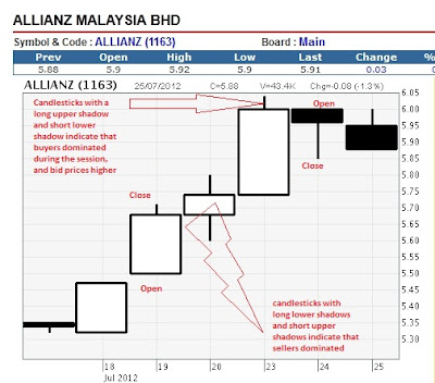
Reading the candlestick charts-

data set that contains open, high, low and close values
Long white candlesticks show strong buying pressure.
Long black candlesticks show strong selling pressure.
Candlesticks with short shadows indicate that most of the trading action was confined near the open and close. Candlesticks with long shadows show that prices extended well past the open and close.